When selecting a neural network architecture, developers often face a choice between maximizing accuracy and managing the computational resources needed to reach it. For those using Python and PyTorch, understanding this balance becomes crucial, especially when models must run on limited hardware or in real-time settings.
Why Model Size and Computation Matter
Many newcomers aim for the highest possible accuracy during neural network training. Yet, a model that edges out another in accuracy might require much more computation, which can make it unsuitable for some deployments. Sometimes, a smaller model with slightly lower accuracy is the better option if it uses far fewer operations.
Experimenting with CNN Architectures on MNIST
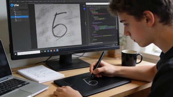
To make this trade-off clear, three convolutional neural networks (CNNs) were trained on the MNIST handwritten digit dataset using Python and PyTorch. The MNIST benchmark includes 70,000 grayscale images of handwritten digits, split into 60,000 for training and 10,000 for testing. Each image is a 28 × 28-pixel square, giving 784 input values, and the task is to classify each as one of ten digits, 0 through 9. The dataset is size-normalized and centered, which simplifies it compared to most real-world computer-vision challenges. Texas Instruments describes MNIST as the industry-standard "Hello World" for handwritten character recognition (Texas Instruments).
All three models use the same basic structure but differ in the number of convolutional channels, which changes both parameter count and computational load.
- Micro CNN: Built for minimal computation, with very few channels.
- Compact CNN: Adds more channels for better feature extraction.
- Wide CNN: Expands channel count to test how much accuracy can be gained.
Each model uses 3 × 3 convolution kernels and follows the same training steps. The main difference is the width of the convolutional layers, letting users see how increasing capacity affects both accuracy and computation. Ertugrul Mutlu notes, “All three use the same basic architecture, dataset, and training procedure.”
Understanding the Architecture and Code
Each CNN takes a 28 × 28 grayscale image through two convolutional layers, each followed by ReLU activation and max pooling. The output is flattened and sent to a fully connected layer that produces ten logits, one for each digit class. This setup follows the standard CNN approach: local pixel neighborhoods are transformed into higher-level features, and pooling reduces spatial resolution. Here is a simplified PyTorch implementation:
class DigitCNN(nn.Module):
    def __init__(self, config):
        super().__init__()
        k = config.kernel
        self.conv1 = nn.Conv2d(1, config.c1, k, padding=k // 2)
        self.pool1 = nn.MaxPool2d(2)
        self.conv2 = nn.Conv2d(config.c1, config.c2, k, padding=k // 2)
        self.pool2 = nn.MaxPool2d(2)
        self.head = nn.Linear(config.c2 * 7 * 7, 10)

    def forward(self, x):
        x = self.pool1(torch.relu(self.conv1(x)))
        x = self.pool2(torch.relu(self.conv2(x)))
        return self.head(torch.flatten(x, 1))
During training, the logits go to CrossEntropyLoss. For inference, softmax turns logits into class probabilities. The predicted digit is the class with the highest probability.
Measuring Computational Cost: Multiply-Accumulate Operations (MACs)
Accuracy is easy to check, but computational cost needs a different metric. Multiply-accumulate operations (MACs) give a hardware-independent estimate of the arithmetic needed for a forward pass. For convolutional layers, MAC count depends on output size, input and output channels, and kernel size. The following Python function calculates MACs for each layer:
def mac_breakdown(cfg):
    k2 = cfg.kernel ** 2
    conv1 = 28 * 28 * cfg.c1 * k2
    conv2 = 14 * 14 * cfg.c1 * cfg.c2 * k2
    linear = 7 * 7 * cfg.c2 * 10
    return {"conv1": conv1, "conv2": conv2, "linear": linear, "total": conv1 + conv2 + linear}
MACs do not cover every operation or hardware-specific optimization, but they offer a clear way to compare arithmetic complexity across architectures. MACs, parameter count, latency, memory use, and energy consumption each measure different sides of model efficiency and should not be swapped for one another. MAC counts estimate arithmetic work, but actual inference time also depends on hardware, memory movement, kernel code, batching, parallelism, and numerical precision. For deployment, benchmarked latency and peak memory on the target CPU, GPU, or microcontroller should back up theoretical operation counts.
Comparing Three CNN Models: Parameters, MACs, and Accuracy
The three models were set up as follows:
ModelConv ChannelsParametersMACs / Image
Micro CNN | 3 → 6 | 3,148 | 55,860
Compact CNN | 8 → 16 | 9,098 | 290,080
Wide CNN | 16 → 32 | 20,490 | 1,031,744
Each model was trained on MNIST using the Adam optimizer, a learning rate of 0.001, batch size of 256, and cross-entropy loss for four epochs. The best checkpoint for each was picked based on validation accuracy, then tested on the official test set. Ertugrul Mutlu explains, “For each model, I selected the checkpoint with the highest validation accuracy and then evaluated it on the official 10,000-image test set.”
Results: Accuracy Gains Versus Computational Cost
After training, the test set results were:
ModelTest AccuracyMACs / Image
Micro CNN | 96.67% | 55,860
Compact CNN | 97.92% | 290,080
Wide CNN | 98.63% | 1,031,744
The Micro CNN reached 96.67% accuracy on the 10,000-image MNIST test set, using 55,860 multiply-accumulate operations per image. The Compact CNN hit 97.92% accuracy at 290,080 MACs per image, so its computational load was about 5.2 times higher for a 1.25 percentage point gain. This shows that accuracy improvements can come at a nonlinear cost: a small test-set gain may need much more arithmetic. These figures are specific to this experiment, not universal benchmarks, since MAC counts and accuracy depend on layer sizes, padding, pooling, preprocessing, and implementation details.
Going from Micro to Compact CNN raised computation by about 5.2 times, with a 1.25 percentage point accuracy gain. The Wide CNN needed roughly 18.5 times more MACs than Micro CNN, but accuracy improved by only 1.96 percentage points. Larger models can bring diminishing accuracy returns compared to their computational demands.
Applying a Computational Budget
To make the trade-off clearer, a hypothetical budget of 75,000 MACs per image was set. Only the Micro CNN fit this limit, achieving 96.67% accuracy. Compact and Wide CNNs went over the budget, showing how resource limits can drive architecture choices. A fair efficiency comparison should separate parameter memory from activation memory. Convolutional parameter count depends on kernel size, input and output channels, and bias terms, while activation memory is set by intermediate feature-map size and batch size. Increasing channel width raises both parameter count and convolutional operations, but pooling can shrink later spatial dimensions and partially limit downstream cost. The fully connected layer can dominate parameter count if the flattened representation is large, so just reporting convolutional channel widths does not fully describe model size.
Interactive Exploration and Visualization
An interactive app was built to let users explore these trade-offs. The browser-based interface, powered by a Python FastAPI backend, lets users pick models, draw digits, check predictions, and see feature maps from the convolutional layers. The app also has an architecture sandbox, where users can change channel counts and kernel sizes to see how these affect parameter counts and MACs—without retraining the model.
Key Takeaways for Learners
- Accuracy alone does not pick the best model for every use. Computational cost can be the deciding factor, especially in limited environments.
- As model capacity grows, accuracy gains often shrink.
- MAC counts help estimate arithmetic complexity, but they do not guarantee faster inference on all hardware.
- Visualizing feature maps helps learners see how CNNs process images and extract features.
- Analytical tools can estimate the cost of hypothetical architectures, but only trained models give real accuracy numbers.
This experiment demonstrates that even small CNNs can perform well on MNIST with efficient computation. For learners using Python and PyTorch, exploring these trade-offs deepens understanding of how architecture choices affect both performance and resource needs. Texas Instruments points out that MNIST is especially useful for teaching because its inputs are small, grayscale, centered, and fixed at 28 by 28 pixels. These features reduce data-loading and preprocessing complexity, letting small CNNs reach high accuracy without large-scale infrastructure. Still, MNIST results should be used as instructional examples, not as proof that the same channel ratios will optimize models for tougher real-world vision tasks.
The full source code, trained model checkpoints, and reproducible results are available on GitHub: Explore Neural Network Efficiency Lab on GitHub.