How Python Calculates Core Loss in Electrical Steel Testing

Engineers and buyers rely on core loss numbers like P1.7/50 = 1.05 W/kg when working with transformer design and electrical steel procurement. These values come from a set of measurements on a standardized test rig called the Epstein frame. Knowing how these numbers are calculated helps engineers and students read mill certificates, compare steel grades, and address supplier questions.

Understanding the Epstein Frame Test

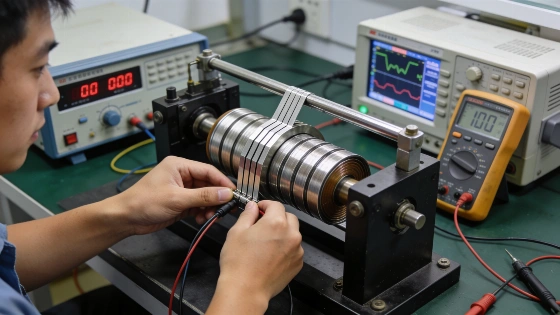
The Epstein frame serves as a standardized lab tool for measuring magnetic properties and specific total loss in electrical steel. Built as a four-bobbin, square fixture, it holds steel strips in a closed magnetic circuit. The setup uses primary excitation and secondary-voltage measurement. The typical 25 cm frame uses strips about 280–320 mm long and 30 mm wide, with overlapping corners to form the magnetic path. This method aims to provide comparable material data for transformer and electrical-machine design. However, the reported loss depends on test conditions, specimen prep, waveform, frequency, flux density, and the chosen standard, so it is not a fixed material constant.

The test follows international standards like IEC 60404-2 and, in North America, ASTM A343. These standards set the measurement framework, including how to configure specimens, excitation, voltage readings, and loss treatment. Always interpret a certificate value with its standard designation and test parameters.

During the test, four main readings are taken:

• Frequency (f): Usually 50 or 60 Hz.
• Average rectified secondary voltage (U2,avg): Sets the flux density.
• RMS secondary voltage (U2,rms): Checks waveform quality.
• Power meter reading (Pm): Shows total power drawn before corrections.

These readings, along with the sample's mass and dimensions, provide the basis for calculating the specific core loss value shown on certificates.

Python Model for Core Loss Calculation

Python can handle this calculation using a data-driven approach. The code below models the Epstein frame sample and processes the readings:

from dataclasses import dataclass

DENSITY = 7650 # kg/m3, conventional density for grain-oriented steel
PATH_M = 0.94 # conventional magnetic path length of a 25 cm Epstein frame
FF = 1.111 # form factor of a pure sine wave (rms / average rectified)

@dataclass(frozen=True)
class EpsteinSample:
    n_strips: int
    length_m: float
    width_m: float
    thickness_m: float

    @property
    def mass_kg(self):
        return self.n_strips * self.length_m * self.width_m * self.thickness_m * DENSITY

    @property
    def area_m2(self):
        # cross-section of ONE limb of the square
        return self.mass_kg / (4 * self.length_m * DENSITY)

    @property
    def active_mass_kg(self):
        # only the steel on the 0.94 m conventional path counts
        return self.mass_kg * PATH_M / (4 * self.length_m)

@dataclass(frozen=True)
class Reading:
    f_hz: float
    u2_avg_v: float
    u2_rms_v: float
    p_meter_w: float

def form_factor(r):
    return r.u2_rms_v / r.u2_avg_v

def peak_polarisation_t(s, r, n2=700):
    # Faraday's law for a sinusoidal flux: U_avg = 4 * f * N2 * A * J_peak
    return r.u2_avg_v / (4 * r.f_hz * n2 * s.area_m2)

def specific_loss_w_per_kg(s, r, ri_ohm, n1=700, n2=700):
    # the meter also measures the power burned in its own voltage circuit
    p_instruments = (FF * r.u2_avg_v) ** 2 / ri_ohm
    p_core = (n1 / n2) * r.p_meter_w - p_instruments
    return p_core / s.active_mass_kg

This model uses several conventions:

• Cross-sectional area comes from mass and density, not direct measurement. This method accounts for coating thickness and strip variation, so the scale is as important as the power analyzer.
• The effective magnetic path is set by convention at 0.94 m. The physical steel length is longer, but the standard uses this value to account for overlapping corners and flux shortcuts.
• Instrument power consumption is subtracted before calculating core loss. The power meter's voltage circuit draws a small but meaningful amount of power, which must be excluded from the final result.

The calculation converts the wattmeter reading to the secondary-referred power scale using the turns ratio, subtracts an instrument-related loss term, and divides the remaining core-loss power by active specimen mass. The instrument correction is (FF × U2,avg)2/Ri, where FF is the form factor and Ri is the relevant instrument-resistance parameter. The corrected specific loss is then Pcore/mactive, giving watts per kilogram.

Example Calculation

Take a sample of 0.27 mm grain-oriented steel, with 24 strips each 280 mm by 30 mm, tested at 50 Hz. The readings are:

s = EpsteinSample(n_strips=24, length_m=0.280, width_m=0.030, thickness_m=0.27e-3)
r = Reading(f_hz=50, u2_avg_v=11.57, u2_rms_v=12.85, p_meter_w=0.384)

print(f"sample mass {s.mass_kg * 1000:.1f} g")
print(f"cross-section {s.area_m2 * 1e6:.1f} mm2")
print(f"active mass {s.active_mass_kg * 1000:.1f} g")
print(f"form factor {form_factor(r):.3f}")
print(f"peak J {peak_polarisation_t(s, r):.3f} T")
print(f"P1.7/50 {specific_loss_w_per_kg(s, r, ri_ohm=10_000):.3f} W/kg")

The output for this sample is:

• Sample mass: 416.4 g
• Cross-section: 48.6 mm²
• Active mass: 349.5 g
• Form factor: 1.111
• Peak polarization: 1.700 T
• P1.7/50: 1.051 W/kg

This means the coil would be certified at 1.05 W/kg at 1.7 T, 50 Hz, which is well below the maximum for a grade like 27Q120 (1.20 W/kg). These figures serve as engineering examples.

Key Checks and Conventions

Two checks matter in any implementation:

• Form factor: The value should be close to 1.111 for a pure sine wave. If the waveform is distorted, the flux is not sinusoidal and the loss calculation is invalid. In that case, the reading should be rejected, not corrected.
• Sample mass: The standard requires a minimum mass (about 240 g) and a strip count that is a multiple of four to keep the frame balanced.

Impact of Path Length Convention

Choosing 0.94 m as the effective path length is a simplification. Studies show the actual effective path can range from 0.90 to 0.96 m, depending on steel grade and test setup. Changing this value in the calculation can shift the reported loss by several percent. This explains why different labs or test methods (like the single sheet tester, IEC 60404-3) may report slightly different results for the same coil. Certificates should always state the test method used.

Comparing International Standards

North American grades are often specified in W/lb at 60 Hz, while European and Chinese grades use W/kg at 50 Hz. Direct comparison is misleading because both the units and the frequency differ. A typical conversion uses a ratio of about 1.32 for grain-oriented steel at 1.7 T:

W_PER_LB_TO_W_PER_KG = 2.2046

def to_w_per_kg_50hz(w_per_lb_60hz, ratio_60_50=1.32):
    return w_per_lb_60hz * W_PER_LB_TO_W_PER_KG / ratio_60_50

print(f"{to_w_per_kg_50hz(0.60):.2f} W/kg") # 1.00
print(f"{to_w_per_kg_50hz(0.70):.2f} W/kg") # 1.17

The unit conversion is exact, but the frequency ratio depends on the steel's properties. Use measured values when available, and treat the ratio as a planning estimate, not a guarantee.

Physical Basis of Core Loss

Electrical-steel losses are usually described as a mix of hysteresis loss, classical eddy-current loss, and additional or anomalous loss components. Eddy-current loss depends on frequency squared, flux-density amplitude squared, and lamination thickness squared. Generalized Steinmetz-type models express core loss using empirical frequency and flux-density exponents. Epstein testing gives measured material data under controlled conditions. Analytical or Python models extrapolate from those data and may not match losses in an assembled transformer or motor. Differences in cutting, burrs, stress, insulation, stacking, and flux direction can cause discrepancies between certificate results and equipment performance.

What the Model Does Not Cover

This simplified model leaves out several factors:

• Air-flux compensation: Some flux passes through air, not steel. Real test frames compensate for this, so the model assumes the voltage reading is already corrected.
• Sample preparation: Shearing and annealing affect loss values, especially for non-oriented steel.
• Built cores: The Epstein frame measures flat strips under low stress. Assembled transformer cores usually show higher losses due to joints, stress, and clamping. The ratio between measured and built core loss is called the building factor.

For more on the Epstein frame method and its comparison with other test approaches, see the official documentation from the International Electrotechnical Commission and ASTM International.